Propensity modeling can be used to increase the impact of your communication with customers and optimize your advertising budget spendings.
Google Analytics data is a well structured data source that can easily be transformed into a machine learning ready dataset.
Backtest on historical data and technical metrics can give you a first sense of your model’s performance while live test and business metrics will allow you to confirm your model’s impact.
Our custom machine learning model outperformed existing baselines: during live tests in terms of ROAS (Return on advertising spend): +221% vs rule based model and +73% vs off-the-shelf machine learning (Google Analytics session quality score).
This article assumes basic fundamentals in machine learning and marketing.
What is propensity modeling ?
Propensity modeling is estimating how likely a customer will perform a given action. There are several actions that can be useful to estimate:
In this article we we will focus on estimating the propensity to purchase an item on an e-commerce website.
But why estimate propensity to purchase ? Because it allows toadapt how we want to interact with a customer. For exemple, suppose we have a very simple propensity model that classify the customers in “Cold”, “Warm” and “Hot” for a given product (“Hot” being customers with highest chance of buying and “Cold” the least):


Well, based on this classificationyou can have a specific targeted response for each class. You might want to have a different marketing approach with a customer that is very close to buying than with one who might not even have heard of your product. Also if you have a limited media budget , you can focus it on customers that have a high likelihood to buy and not spend too much on the ones that are long shots.
This simple type of rule based classification can give good results and is usually better than not having any but it has several limitations:
To cope with those limitations we can use a more data driven approach: use machine learning on our data to predict a probability of purchase for each customer.
Understanding Google Analytics data
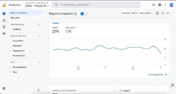
Google Analytics is an analytics web service that tracks usage data and traffic on website and applications.

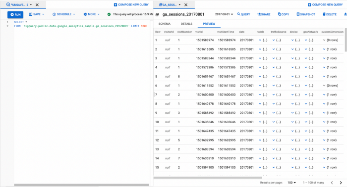
Google Analytics data can be easily exported to Big Query (Google Cloud Platform fully managed data warehouse service) where it can be accessed via an SQL like syntax:

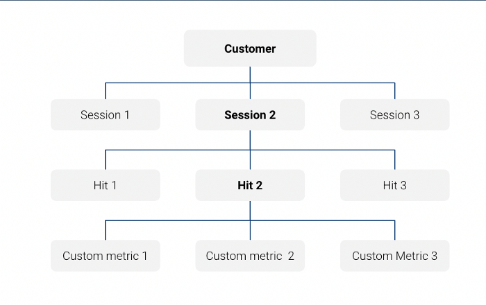
Note that the Big Query export table with Google Analytics data is a nested table at session level:

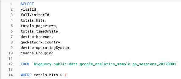
For example in this query we are only looking at session level features:


And in this query we have used an Unnest function to query the same information at hit level:
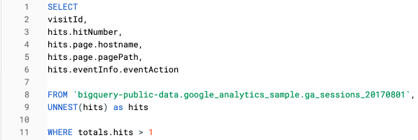


For more information on GA data check the documentation. Note that our project was developed on GA360 so if you are using the latest version, GA4, there will be some slight differences in data model, especially the table will be at event level. There are public sample tables of GA360 and GA4 data available on Big Query.
Now that we have access our raw data source we need to perform feature engineering before we can feed our table to a machine learning algorithm
Crafting the right features
The aim of the feature engineering step is to transform the raw Google Analytics data (extracted from Big Query) into a table ready to be used forMachine Learning.
GA data is very well structured and will require minimal data cleaning steps. However there are still a lot of information present in the table, many of which are not useful for machine learning or cannot be used as is so selecting and crafting the right features is important. For this we built features that seemed to be the most correlated with buying a product.
We crafted 4 types of features:
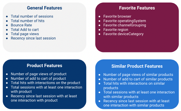

Note that we are computing all those features at a customer level which means that we are aggregating information from multiple sessions for each customer (using fullVisitorId field as a key)
General Features
Global features are numerical features that give general information about the session.
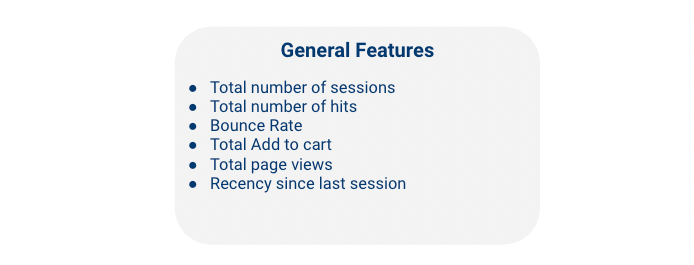

Note that bounce rate is defined as % of times the customer only visited only one webpage during a session.
It was also important to include information on the recency of events: for instance a customer that just visited your website is probably more keen to purchase than one that visited it 3 months ago. For more information on this topic you can check the theory on RFM (recency, frequency monetary value).
So we added a feature Recency since last session = 1 / Number of days since last session which allows the value to be normalized between 0 and 1
Favorite features
We also wanted to include some information on the key categorical data available such as browser or device. Since that information is at session level, there can be several different values for a single customer so we only take the one that occurs the most per customer (i.e. the favorite). Also, to avoid having categorical features with too high cardinality, we only keep the 5 most common values for each feature and replace all the other values with an “Other” value


Product features
While the first two types of features are definitely useful in helping us answer the question “Is a customer going to buy on my website?”, they are not specific enough if we need to know “Is the customer going to buy a specific product?”. To help answer this question we built product specific features that only include the product for which we are trying to predict the purchase:
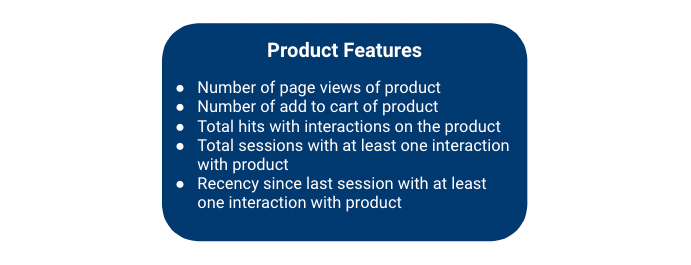

For Recency since last session with at least one interaction with this product, we use the same formula than for the Session Recency in the General Features. However we can have cases where there is 0 session with at least one interaction with the product, in which case we fill with 0. This makes sense from a business perspective since is our highest possible value is 1 (when the customer had a session since yesterday).
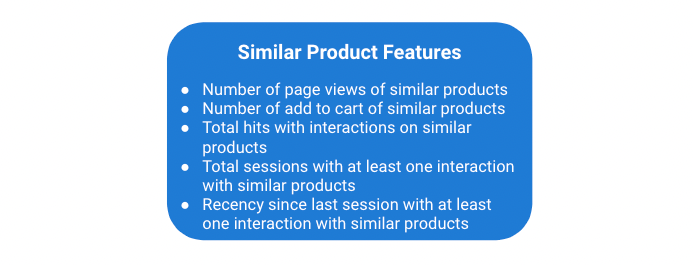
Similar Product features
In addition to looking at the customer’s interaction with the product for which we are trying to predict the probability to purchase, knowing that the customer interacted with other products with similar function and price range can definitely be useful (ie substitute product). For this reason we added a set of Similar Product features that are identical to the Product features except that we also include similar products in the variable scope. The similar products for a given product were defined using business inputs.

We now have our feature engineered dataset on which we can train our machine learning model.
Training the model
Since we want to know whether a customer is going to purchase a specific product or not, this is a binary classification problem.
For our first iteration, we did the following to create our machine learning dataset (which was 1 row per customer):


However some first data exploration quickly showed that there was a strong class imbalance issue: Class 1 / Class 0 ratio was over 1:1000 and we did not have enough Class 1 customers. This can be very problematic for machine learning models.
To cope with these issues we made several modifications in our approach:
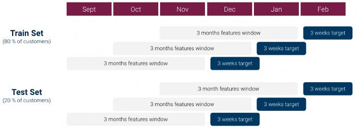

Using this dataset we tested with several classification models: Linear Model, Random Forest and XGboost, finetuning hyperparameters using grid search, and ended up selecting an XGboost model.
Evaluating our model
When evaluating a propensity model there are two main types of evaluations that can be performed:
Backtest Evaluation
First we performed backtest evaluation: we applied our model to past historical data and checked that our model is correctly identifying customers that are going to perform an add to cart. Since we are using a binary classifier, the model produces a probability score between 0 and 1 of being Class 1 (Add to cart).
confusion matrix and compute the precision / recall (or their combined form in thef1 score). However there are two issues with these simple metrics:


So we decided to use two metrics that were more interpretable:
Results on those metrics were rather positive, especially, Uplift was around 13.5.
Backtest evaluation is a risk free method for a first assessment of a propensity model but it has several limitations:
Livetest Evaluation
So to get a better idea of our model’s business value we need to perform live test evaluation. Here we activate our model and use it to prioritize advertising budget spendings :
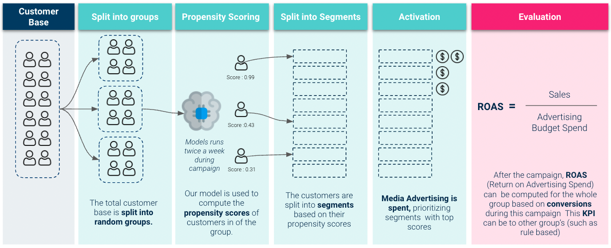

Results we obtained on the livetest were very solid:
Conclusion
In addition to reaching solid performance, a strong side benefit of our approach is that our feature engineering is very generic. Almost none of the feature engineering steps need to be adapted to apply our model to a different country scope or product scope. In fact following our first success in the livetest, we were able to roll out our model to multiple countries and products in a very efficient manner.
Thank you for reading. I would be glad to hear your comments on this approach. Have you ever build propensity models? If so, what did you do differently?
Thanks to Bruce Delattre, Rafaëlle Aygalenq, and Cédric Ly.


