Until now we have mainly talked about forecasting regular products that have been on the shelf for quite some time. But what about products that have been very recently launched ?
In this article we will show you how we tackled this issue by proposing an alternative solution to our boosting model based on product look-alikes.
It consists of training a clustering model on old innovations to detect sales pattern similarities, then mapping that to product characteristics with a classification model and then inferring the sales of new innovation with simple statistical methods based on the outputs of model 1 and 2.
Why is forecasting launched products so hard ?
A bit of context
Product launches are very common in retail. It is in CPG companies’ nature to diversify their products. They want to appeal to their customers and adapt their products to behavioural changes. And the company we did the project for was no exception, they nearly release 50–60 innovations (new products) every year.
We define an innovation as being rather a new brand of product being launched or a new product with a new flavour being introduced to an already existing brand. After a certain time (for instance, in our case, 2 months) an innovation becomes a regular product.
There are other cases where a new product code can be generated like
We do not consider these cases as innovations but renovations and therefore they are out of our scope.We had access to product launches with sales data from 2017 to 2019, so roughly 150 innovation products.
The main challenge
Our job was to make weekly forecasts for the 14 weeks ahead at warehouse/daily/product level.
The first time the model had to be applied was 7 days after its launch, meaning it would only have 7 days of historical data and had to predict sales for the coming 14 x 7 = 98 days ! The last time we had to apply the model was 60 days after the launch. This means that a launched product would be considered as a “regular product” after 2 months since it would have achieved some “stability” in its sales cycles, but of course, this will depend on your company’s activity and product nature. After this 2 months phase, the core model (model developed for regular products) would take over the innovation model and make forecasts for the given launch, this decision was validated by the business teams that had some knowledge on the sales cycles of innovations.
Very limited historical data
The amount of historical data at our disposal is critically low for making accurate forecasts. We have a training dataset which is much smaller than our prediction/test dataset and that often brings very poor forecast accuracy. We are talking about having a few weeks in training data and having to make forecasts for 98 days.
Launched products have very unstable sales at the beginning
Besides, sales data are often very messy during the first weeks of launch as trends can dramatically change. In fact retailers order huge quantities of the innovation in the first 2 weeks to fill in their shelves, they call this the fulfillment phase. After that orders drop generally on W3 and W4 and then they increase a bit.
Again, here a lot can happen : some retailers might realize that the new product is not selling very well during the first weeks in its stores and therefore drastically reduce its orders as a quick reaction. Or a product might have huge volumes of orders from some retailers that the manufacturer might not be able to fully fulfill because they did not anticipate this level of demand. The retailers will keep ordering high volumes during the following weeks to compensate for the volumes for which they were not fully delivered.


All the elements listed above are a clear explanation of why predicting innovation sales is hard and therefore why we had to develop a specific model for these products.
Evaluation criteria
We had the same evaluation metrics as for regular products (W+1 and W+2 Forecast Accuracies at national/weekly level). As a reminder here is the formula of a forecast accuracy:


We added another dimension to this problem. We calculated these metrics for each prediction date (the date at which we make our prediction) with regards to the launch date.
We monitored W+1 and W+2 forecast accuracies for prediction dates going from D+7 until D+49, meaning that our scorecard would look like this:
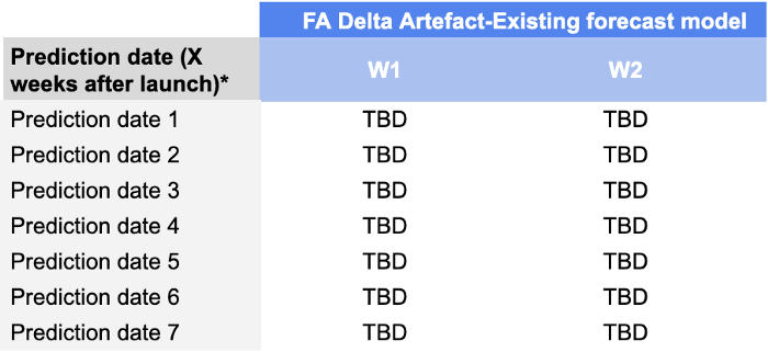

The reason we added this dimension is that it is really important to demand planners to monitor the performances of their forecasts during the first weeks of launch. A model that provides good quality forecasts during the first weeks enables them to avoid big replenishment issues (that are common after the launch due to uncertainty) and ultimately succeed in their launch.
Proposed approach
Why did classical ML provide poor results ?
As said before we have a “small data” problem. The small size of our training data and its very erratic nature makes it unsuitable for a machine learning model.
Most often, boosting models require 2–3 years of historical sales data to detect general trends/seasonality effects and at least 2–3 months of Time Series data for one product to make “accurate predictions”. This was not the case for us; our XGBoost model would only see a few weeks of historical sales for each product.
We trained an XGBoost model on innovation products with the following logic
And the results were not good at all ! Therefore we decided to completely change our approach for these products.


Classical Time Series models did not save the day either
Since our first iteration with XGBoost was a total failure, we decided to try our luck with some good old-fashioned time series models (VARMA, SARIMAX, Prophet, etc). Time Series models have the virtue of being simpler and easier to interpret than boosting models. Also, since they are trained on one product, they can more easily adapt to abrupt trend changes.
The idea was to train one model (a Prophet model for example) per product that would make forecasts at national/daily level. Like above, the model would be trained several times too, each time until the day before the prediction date (D+7, D+14, etc) and make forecasts for the 14 week horizon.
But here, like above, the results were still not satisfactory and the reason was pretty much the same: not enough historical data ! The history was too shallow and the data was too messy for the model to understand a clear pattern and make accurate predictions.


Product clustering based on look-alikes : the Messiah
With our two first attempts at making forecasts being inconclusive, we decided to go completely in another direction.
We analyzed the sales of all innovations from 2017 to 2019 and realized that many had similar sales curves during the first months of their respective launches, this gave us the idea to make forecasts based on product similarities with old innovations. Our intuition was strengthened since we found some research papers of other fellow data scientists suggesting a similar approach (1).
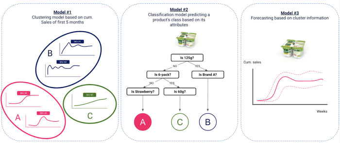
Our approach consisted of 3 fundamental steps
Clustering of old innovations based on sales — Data scope : Innovations launched from 2017 to 2018 included
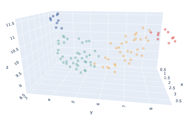
The idea is to cluster old innovations based on their time series curve into groups of similar products. Products being in the same cluster have similar sales patterns and therefore the sales of a single innovation can be deduced from knowing the sales of older innovations.
Our input data was the MinMax normalized cumulative sales of old innovations during their 5 first months. We looked at cumulative sales because we wanted our clustering model to get a sense of when each product would reach its regular sales pace. We normalized the cumulative sales because some products had the same curve shape but different sales volume and we wanted to put them in the same cluster as we focus here on similarity.
We clustered our products with a K-Means model with the K parameter being chosen automatically through a benchmark using the Silhouette index.The optimal number was K=4.We also tried different distance metrics between euclidean and DTW, with euclidean giving more satisfactory resultats during our tests.



Classification model predicting a product’s cluster based on its attributes — Data scope : Innovations launched from 2017 to 2018 included
The idea here is to find a link between the cluster the product belongs to and its attributes, like dimension, brand, flavour, etc, as well as some contextual data like launch period, media campaigns, etc. That link would be found with the help of a classification model.
The model would be fed with product attributes alongside with contextual data and it would try to predict an innovation’s cluster based on that. The intuition behind this approach is to see if we can answer the following question :
If we know an innovation’s attributes + contextual data in advance, can we predict the kind of sales behaviour this product will have after its launch ?
Since we had very limited data (roughly 100 products), we trained a simple BaggingClassifier on our products with a 75%-25% train/test split. We ended up with a F1 score of 84% on the test set.
We performed some analysis on product attributes to see if we can find some business explanation for each cluster and here are our findings:
Forecasting new innovations sales based on predicted clusters — Data scope : Innovations launched after 2019
Now that we are able to link an innovation’s sales to its attributes, we can apply our model to new innovations to determine their cluster and hence predict their sales.
We started very simple. For each new innovation (launched after 2019), we calculated the average sales of old innovations (launched before 2019) that were in the same cluster as the new one, during their first weeks of launch and considered that as our forecast for the new innovation.
This simplistic approach was actually a good start but had one major flaw : We were able to accurately predict the shape of the new innovation, however the scale of our prediction was not good.
We decided to scale our predictions by comparing the sales of the new innovation and the old similar ones from D+0 until the prediction date (prediction date). Since sell-out data was as insightful as sell-in data in predicting future sell-in in our case, we calculated 2 scaling coefficients, one with sell-in and one with sell-out.
Sell-in coeff = average sell-in of old similar innovations until prediction date / average sell-in of new innovation until prediction date
Sell-out coeff = average sell-out of old similar innovations until prediction date / average sell-out of new innovation until prediction date
We finally upscaled/downscaled our predictions with the mean of these 2 coefficients.

Results & conclusions
Here are our results on each prediction date and prediction horizon:
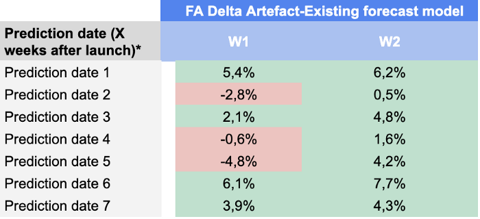

We were quite satisfied with these results as our model was able to beat demand planners’ forecast in almost every KPI until prediction date 49.
References
1. New Product Forecasting with Analogous Products<
I would like to thank everyone who has worked on this project, specially Sylvain Combettes, without whom this article would have never been written>
And thank you for reading that far! I would be glad to hear your feedback. If you enjoyed the read, feel free to check our open positions at Artefact 🙂

